A World of Causal Inference with EconML by Microsoft Research
Introduction
That was one of the surprising headlines that the study “An experimental approach to alleviating global poverty” was awarded for the Novel prize Economics in 2019 for Abhijit Banerjee, Esther Duflo, and Michael Kremer. It’s said that they had introduced new approach and standard to obtain reliable ways to identify causal relationships from microdata of in development economics, even when relationships observed in microdata sometimes suffer from confounding effects. RCT (Randomised Controlled Trials) technique was added in their study for identifying causal relationships, which is one of well-known methods that was born in scientific and medical fields in the past and it’s been seen freqently in EBPM (Evidence Based Policy Making) scene recent years. [1]

The Laureates’ research findings — and those of the researchers following in their footsteps — have dramatically improved our ability to fight poverty in practice. As a direct result of one of their studies, more than five million Indian children have benefitted from effective programmes of remedial tutoring in schools. Another example is the heavy subsidies for preventive healthcare that have been introduced in many countries.
In this article I will cover a little extensive area in context of causal inference in statistical and machine learning, additionally introduce a Python EconML package by Mirosoft Research, which consists of some machine learning techniques for econometrics to bring automation to complex causal inference problems in specific area. This is an investigation of overview for myself to undertake researches about the recent studies of causal inference and explore the possibilities of a case to use EconML package for actual causal studies.
Disclaimer: This article contains links to third-party websites or other content for information purposes only (“Third-Party Sites”). The Third-Party Sites are not under the control of me, and its affiliates, and I am not responsible for the content of any Third-Party Sites, including without limitation any link contained in the Third-Party Sites, or any changes or updates to the Third-Party Sites. I am providing these links to you only as a convenience, and the inclusion of any link does not imply endorsement, approval or recommendation by me of the site or any association with its operators.
RCT (Randomised Controlled Trials)
Let’s get started from RCT (Randomised Controlled Trials) but I don’t go over too much details of RCT itself here with regards to causal inference. Because it’s the too long winding road to trace from the beginning to the present place in history. There are a lot of stories published for you to check how this technique was found and how have this experiment been polished from the first report of James Lind in 1747 to identify treatment for scurvy and later in agriculature field, due to Jerzy Neyman and Ronald A. Fisher. Fisher’s experimental research and his writings popularized and familiarized randomized experiments specifically in public as said. [2]
Let’s train ourselves with the basic knowlege of RCT first. How RCT works is explained in the name clearly. It’s relevant to Randomized, Controlled, and Trials. Let’s take a population for an experiment with a certain hypothesis. We can split it into multiple groups, let’s say we have two groups labeled “treatment” and “control” with ramdom pick-up from the population. The former group “treatment” has an intervention being assessed while the latter group “control” has an alternative condition (placebo for mecidal cases mostly), or no intervention at all. RCT goes like this. Under the Randomized groups eluding selection bias and allocation bias, experimental interventions for the Controlled group could show how effective the Trials did. Treatment efficacy can be assessed in comparison to the controlled. Here’s a good article for medical case RCT with easy-for-reading explanations. [3]
Randomization is crucial in RCT to avoid confounding effects. Treatment efficacy in RCT can be maximized when fairness in groups is achieved with randomization by avoiding selection bias and allocation bias to obtain satisfactoy preconditions. Once a trial has started it’s important to employ “blinded trials” to avoid to skew its result for participants, experimenters and assessors. RCT has scored five points that is the most robust method on the Maryland SMS (Scientific Methods Scale). It’s assessed of whether an evaluation provides convincing evidence on policy impacts. RCT can be said that one of credible statistical causal inference methods for conducting policy making there by reducing spurious causality and bias in systematic reviews since it’s invented for the sake of clinical trials. [4]
There are frequently cited drawbacks of RCT such as expensive cost and time, ethical proglems, conflict of interests, etc. First of all, there could be some variances between groups because a fair randomization is not achievable sometimes, and people in treatment group can’t be obliged to take a treatment so they can pretend taking that treatment on the surface, which would change experiment result dramatically. It also does not care about varying treatment effect across sub-groups in assigned groups and between individuals also (some attributes in individuals could be considered). So next I will cover some other causal inference methods to tackle those RCT’s drawbacks or that those can bypass the problems and how to select a technique for your purpose before an introduction of EconML library.
Causal inference
Conducting RCT experiment needs expensive cost and time then the experiment can produce experimental data with that sacrifice. You might already notice that ideal RCT approach needs experimental data while some profound methods work with observational data (Rubin causal model is one of the statistical approaches for observational studies with the assumption of potential outcome). Legit experiment data can’t be obtained sometimes for some reasons and estimating the treatment effect could be feasible when a randomized controlled experiment is not possible. Because of? Due to the noisy nature of experiment data, such as high variance in the data, or when some people in a treatment group did not receive the treatment or when true randomization for groups was simply not possible.Also we may want to know varied effectiveness across sub-groups in assigned groups or individuals for more personalized policy or service in purpose. There are a variety of causal inference methods not only statistical RCT approach but others too to tackle with those RCT’s drawbacks or to address additional complexities within experimental data and observational data for giving us more insight into the treatment effect as a result.
Uber Engineering published a quite useful article regarding how to choose a causal inference method for both experimental data and observational data cases. If you look through the article you would get an overview about a variety of methods that have been adopted already in Uber Engineering and how the techniques have improved the analysis of experiments at Uber, quasi-experiments, and observational data. Causal inference is becoming an intersection of statistical approach and machine learning technique with a variety of methods that we can find those in the flowchart to grasp the overview here. The flowchart is said not so exhaustive but looks easy to understand if-nots cases for experimental data at a glance. [5]
Causal inference methods

Look at the top left box. As aforementioned the first significant drawback in RCT seems the requirement for fair-enough randomization with proper methods. It’s expected that a population is assigned into groups randomly in RCT. Due to the noisy nature of experimental data there might be always pre-existing differences across assigned groups. There are some methods to cope with the pre-existing problems such as adjusting pre-existing difference by reducing variance in data or treating the experiment as an observational study to know causal relations under such circumstance. I’ll introduce Propensity score matching for your reference and other three’s links.
Let’s think about a difference of a number of samples in treatment and control groups. Image we have selected 100 people for treatment group and 900 people for control group from 1000 people in total (a population). There might be selection bias for those 100 people in the treatment group and the treatment effect will be confounded with the effect of the covariates from bias. Propensity score matching can reduce this kind of bias due to confoundings that might be found in an estimate of the treatment effect obtained from simply comparing outcomes among units that received the treatment versus those that did not receive the treatment.
But how? Propensity score is basically a predicted probability (by logistic regression) of group membership for treatment versus control group — based on observed predictors. In other word this is a probability each participant could be in the treatment group with respect to the confounders. Now we can use the propensity score for matching that is to select one participant in the treatment units to one or more non-participant from the comparison units based on propensity score. Caliper matching with one-to-one allocation is general (comparison units within a certain width of the propensity score of the treated units get matched).
If there is no pre-existing difference in assigned groups we would need to consider if the treatment effect is trustworthy or not because some people in the treatment group might not have received the treatment either consciously or unconsciously. For example, some people who were assigned into the treatment group received medicine but they actually didn’t take that medicine for some reasons. They were not the actual treated but counted as members of the treatment group. So the estimated effect would be diluted because some of the people in the treatment group were not actually treated. This is the case. Here what we want to know is the treatment effect for people who took the treatment if and only if they were assigned to the treatment group. These people are called Compliers in this study (Joshua D. Angrist, Guido W. Imbens and Donald B. Rubin 1996). On the other hand Non-compliers consists of other three of four sub-groups (Never-taker, Always-taker, Defier) if we can assume exclusive restriction.
- Compilers — Induced to take the treatment by assignment to the treatment
- Never-taker — Does not change status with the assignment, avoider
- Always-taker — Take the treatment regardless of the assignment, volunteer
- Defier — Do the opposite of their assignment, avoid to take the treatment by assignment or induced to take the treatment by assignment to the control group
CACE (Complier Average Causal Effect) or LATE (Local Average Treatment Effect) are ATE (Average Treatment Effect) of compliers who are the subnet of the population that are induced to take the treatment if and only they were assigned to the treatment group. Under imperfect compliance situation it’s not possible for us to identify ATE (Average Treatment Effect) directly. Instead of that estimating CACE/LATE as an observational sturdy becomes more feasible option within RCM (Rubin causal model). It can be estimated by a ratio of the estimated ITT (Intention-To-Treat) effect and the estimated proportion of compliers, or alternatively through an instrumental variable estimator. [6]
At the third box from the left this is the case if effectiveness vary across sub-groups in assigned groups or individuals, or maybe some segments exist in sub-groups in both treatment and control groups. For example, in RCT there is no concept of considering attributes such as sex, age, or some segments for those treatment and control groups. Because a randomization is expected to assign a population into sub-groups by maximizing statistical effect, minimizing selection bias and confounding with the effect of the covariates. For example, imagine we want to know the treatment effect of e-mail from the company to its customers to avoid cancellation of the service (like lower churn rate of phone contract). It’s important to know what sort of people (attributes) might decrease their likelihood to churn. It seems not predictive analysis we have seen in machine learning models but more prescriptive analysis how the treatment might have changed the outcome for specific sub-groups or individuals. Heterogeneous treatment effects are effects of an intervention on an outcome of interest for a sample with a particular set of features and usually involve CATE (Conditional Average Treatment Effect) calculation. CATE (Conditional Average Treatment Effect) is an average treatment effect specific to a sub-group of subjects, where the sub-group is defined by some attributes (e.g. the ATE among female individuals) or attributes of the context in which the experiment occurs (e.g. the ATE among individuals at a specific site in a multi-site field experiment). Uplift modeling and Quantile regression are also intoroduced in the article for estimating Heterogeneous treatment effects.
As we looked through there are a variety of methods from experimental to observational study to know or estimate causal relations and causal effects for specific situation. It’s crucial to foresee what problem and treatment effect exactly you would want to investigate from data beforehand. Heterogeneous treatment effects are useful to not predict the outcome but to estimate how the treatment might have changed the outcome for specific sub-groups, a group with a particular set of features, attributes with calculation of CATE (Conditional Average Treatment Effect) in analysis. Uplift modeling on the other hand needs A/B experimental test data to train a model then use that to identify the optimal treatment for different segments based on the results.
EconML Introduction
ALICE (stands for Automated Learning and Intelligence for Causation and Economics) is a project led by Microsoft Research and the implementor of EconML package that is usefull handy tool for estimating CATE (Conditional Average Treatment Effect) from observational data. [7]
EconML is a Python package for estimating heterogeneous treatment effects from observational data via machine learning.
There are multiple methods implemented for estimators and these estimators fall under two main categories, the one leverages machine learning techniques in various ways for estimating Heterogeneous Treatment Effects such as in Double Machine Learning, Doubly Robust Learing, and Orthogonal Random Forests (Forest Based Estimators), and the one uses meta-algorithms which consist of the base learners (Random forest, Linear regression, etc) dealing with control and treatment groups separately and a meta-level which can be viewed as a function of the base learners, in Meta-learners. [8]
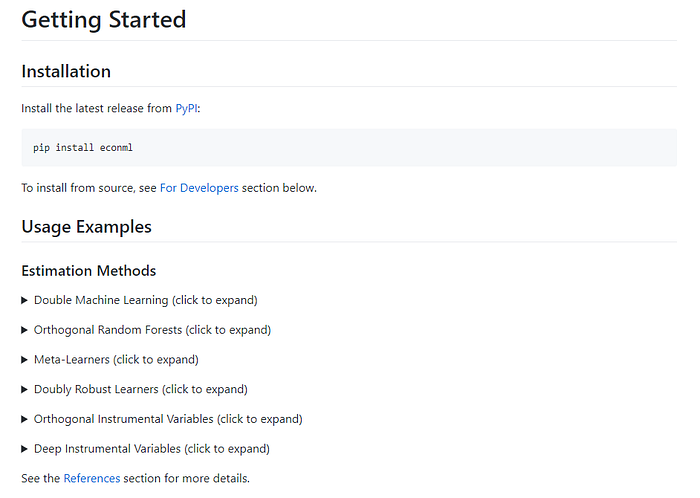
Installing EconML is straightforward, just run pip command as follows. There is a container image that has econml package based on Anaconda3 or a Dockerfile with notebooks in github repository. You can either install the package by pip or clone the code to local and build it for testing.
# install econml package
$ pip install econml# use docker image
$ git clone git@github.com:yuyasugano/econml-test.git
$ docker build -t econml .
$ docker run -p 3000:8888 -v ${PWD}/notebooks:/opt/notebooks econml
conda list in the container shows library versions below as of writing. econml 0.7.0 was built in this container.
econml                    0.7.0                    pypi_0    pypi
numpy                     1.16.0                   pypi_0    pypi
scikit-learn              0.21.2           py37hd81dba3_0
scikit-image              0.15.0           py37he6710b0_0
pandas                    0.24.2           py37he6710b0_0
h5py                      2.9.0            py37h7918eee_0
tensorboard               2.1.1                    pypi_0    pypi
tensorflow                2.1.0                    pypi_0    pypi
tensorflow-estimator      2.1.0                    pypi_0    pypi
If you’d like to use these fixed versions for required libraries, do not create an image yourself but pull the built image from DockerHub instead. [9]
If you did volume mount with -v ${PWD}/notebooks:/opt/notebooks you would have the sample notebooks already in hand. There are two informative case studies under the CustomerScenarios directory, the one is to estimate the heterogeneous price sensitivities that vary with multiple customer features for learning what sorts of users would respond most strongly to a discount for media company case, and the one is to understand the heterogeneous treatment effect from a direct A/B test but under imperfect compliance by tackling with some shortcomings of the characteristic for travel company case.

If you get lost in the maze of selections of methods the given flowchart is helpful to identify what class in the library would satisfy your requirements in user guide page. [10]

As we looked through here’s the intersection of statistical approach and machine learning technique for various areas and industries to help decision-makings in policy and business nowadays. EconML is rich and useful tool set to estimate CATE (Heterogeneous treatment effects) from observational data for specific sub-groups or people who have particular attributes or features, which is good. However using these methods from classic method such as RCT to relatively recent EconML library needs extensive expertise in statistical and machine learning and more deep knowledge for us to understand right use in right place. It was not realistic to cover causal inference throughly here. Therefore it might be superficial but I hope this little article opens a door to a world of causal inference for you.
Reference
- [1] Press release: The Prize in Economic Sciences 2019
- [2] Wikipedia — Randomized Controlled Trial
- [3] What is Evidence? | Randomised controlled trials
- [4] Guide to scoring methods using the Maryland Scientific Methods Scale
- [5] Using Causal Inference to Improve the Uber User Experience
- [6] Wikipedia — Local average treatment effect
- [7] ALICE (Automated Learning and Intelligence for Causation and Economics) — Microsoft Research
- [8] microsoft/EconML
- [9] suganoyuya/econml
- [10] EconML User Guide — Library Flow Chart
- [11] A World of Causal Inference with EconML by Microsoft Research

